Economic terminology
Quotes from Jackson & McIver, "Microeconomics", edition 8, McGraw-Hill-Irwin 2009, ISBN 978-0-074-7169-1 are marked thus.
Quotes from the Uni SA website are marked thus.
Quotes from Bredon G, 2008, "Study Guide to Accompany Microeconomics by Jackson and McIver", edition 8 revised, McGraw-Hill-Irwin, ISBN 978-0-0701-6027-9 are marked thus.
Quotes from the course notes are marked thus.
Stuff that I've said and I'm really unsure that are right are marked thus.
Draw a diagram for most, if not all, exam questions
Students must not forget 3 main things when answering a question:
- Always use economic concepts eg defining price elasticity of demand.
- Use examples, graphs/models, tables etc to support your argument.
- Finally, make sure you have answered the question.
- Symbols and Acronyms
-
Symbols used throughout:
- Economics
-
The study of the allocation of scarce resources. The efficient use of limited productive resources for the purpose
of attaining the maximum satisfaction of our material wants.
Economic problem: unlimited material wants versus limited resources.
- Economic problem
-
Unlimited or insatiable wants of society for goods and services that give utility
compared with the fact that Economic resources are limited or scarce
.
Expressed by 5 fundamental questions:
- How much total output is to be produced?
- What combination of outputs is to be produced?
- How are these outputs to be produced?
- Who is to receive or consume the outputs?
- How can change be accomodated?
Or, by the lecturer, 3 fundamental questions:
- What to produce? (Consumers decide, price is important)
- How to produce it? (Business decide this, by "profit maximizing, cost minimizing", least price N, L, K)
- For whom to produce it for? (Those who have the ability and willingness to pay the market price)
Price mechanism is key to solving economic problem. Prices are reviewed (set) in the market,
therefore we are a market economy.
- Applied economics
-
Formulating policies for correcting the problem
under scrutiny
Also known as "policy" economics.
- Empirical economics
-
Also called Descriptive Economics. Gathering facts relevant
to an economic problem. Somewhat related to positive economics?
- Positive economics
-
Deals with facts (and theories about these
facts) and avoids value judgements. Attempts to set out scientific statements about economic
behaviour.
That is, "just the facts, ma'am".
- Normative economics
-
Based upon someone's value judgements about
what particular policy action should be recommended, based on a given economic generalisation or
relationship. It embodies subjective feeling about "what ought to be"
ie: the outcome
of this is applied economics. Hint, think of this as "What should
be normal".
- Inductive reasoning
-
Using facts to produce a generalisation. Compare to deductive reasoning.
- Deductive reasoning
-
Reasoning from assumptions to conclusions
by testing a hypothesis
or generalisation.
- Ceteris Paribus
-
"All other things being equal". The assumption that other things are held at
steady state, that it is only the factor we are looking at that is influencing the
result, ... that all other variables, other than the one being considered, are constant
. This is usually a valid assumption to make, but not always.
Done to simplify the maths.
Abbreviated as "cet. par.".
In the exam, preface most of your answers with "Assuming cet. par., ..."
- Reasoning pitfalls
-
- Bias
- Loaded terminology: using emotive words, for example
- Definitions
- Fallacy of composition: what is true for the individual is not necessarily true for the
group.
- Cause and effect: correlation does not imply causation, and something following another thing
does not necessarily mean that the first thing caused the second.
- Economic quackery
- Macroeconomics
-
Economics on a grander scale than microeconomics. Looks at the economy as a whole, or in terms of the
aggregates (a collection of specific economic units that are treated as one huge unit,
eg: the approximately seven million households in the economy, the government, the business sector etc).
The branch of economics that studies the entire economy, especially such topics as aggregate production, unemployment, inflation, and business cycles. It can be thought of as the study of the economic forest, as compared to microeconomics, which is study of the economic trees.
- Microeconomics
-
The study of the behaviour of economic units, e.g.: companies
- Economic goals
-
These are values that are widely (although not universally) accepted in our society as things worth pursuing economically.
Note that some are complimentary, some are conflicting.
- Economic growth
- Full employment
- Economic efficiency - maximum benefit from minimum cost
- Price-level stability (that is, low or no inflation or deflation)
- Economic freedom - consumers, businesses and workers allowed a high degree of freedom to conduct economic activities
- An equitable distribution of income
- Economic security - provision for those that can't otherwise earn sufficient income
- External balance - international trade to be evenly split between exports and imports
Complimentary goals: Full employment (2) means that low incomes are avoided (6) and improves economic security (7).
Economic growth (1) may lead to a more equal income distribution (6).
Conflicting goals: These usually need to involve trade-offs. Societies must decide where to draw the line on these.
Some economists say that economic growth (1) and full employment
(2) may lead to strong inflation (4). Full employment (2) may drop economic efficiency (3) due to employers opting for labour rather
than capital (especially technologies) to produce.
- Marginalism
-
Analysis of the changes in production. For example, if we make one more widget, what is the benefit? What is the opportunity cost?
- Utility
-
The economist's term for "satisfaction". Satisfying our material wants results in utility.
- Horizontal and vertical axis
-
In economic graphs, the determining (independent) factor is set as the horizontal (x) axis, the dependent factor on the
vertical (y) axis.
- Direct and inverse relationships (positive and negative)
-
Direct relationships are where the two factors change in the same direction, i.e.: the graph has a positive slope. An inverse
relationship goes the other way (negative slope).
- Independent and dependent variables (cause and effect)
-
The independent variable is the cause, the dependent variable the effect. For example, generally the more income you make, the
more you consume. In this case, the income causes the consumption, not the other way around, so the income is the independent
variable, and the consumption is the dependent variable.
- Slope (negative and positive)
-
Positive: bottom left to top right. Negative top left to bottom right.
- Tangent
-
A straight line that touches a curve at a certain point. The straight line has the same
slope as the curve at that point.
- Limited resources
-
All resources are limited. There is only so much land, muscle and brain power, and capital available to produce.
- Scarcity and choice
-
The heart of economics. Resources are limited, and so a choice must be made on what
to produce, in what quantities and for whom.
- Resources
-
Land and capital are property resources, while labour and entrepreneurial ability are
human resources.
- Land (N)
-
All the natural resources available to us, eg: minerals, land, sunshine, air, earth etc.
Income from these resources is known as rental.
- Labour (L)
-
Muscle and brain power available to produce.
Income from labour is known as wages.
- Capital (K)
-
(Das Kapital?) The manufactured things we use to help us produce and distribute a product. For example, to produce a meal,
a chef would use various items of capital such as a frying pan, a stove, a restaurant etc.
The process of procuring capital is known as investment.
Also known as investment goods
Some texts have Technology as a special part of labour.
Income from supplying capital is known as interest.
Does not refer to money!
Money as such produces nothing, and is not
an economic resource
- Entrepreneurial ability/enterprise
-
Really a part of labour, but a special part, treated differently in some texts. The human
resource that combines the other resources to produce a product, make non-routine decisions,
innovate and bear risk.
Income due to enterprise is known as profit. Of course, a negative profit
is a loss. Profit/Loss = TR - TC
- Opportunity cost
-
Also known as economic cost.
The cost of the best alternative forgone. The highest valued
alternative foregone in the pursuit of an activity. This is a hallmark of anything dealing with
economics -- and life for that matter -- because any action that you take prevents you from doing
something else. The ultimate source of opportunity cost is the pervasive problem of scarcity
(unlimited wants and needs, but limited resources). Whenever limited resources are used to
satisfy one want or need, there are an unlimited number of other wants and needs that remain
unsatisfied. Herein lies the essence of opportunity cost. Doing one thing prevents doing
another.
It is what you sacrifice to do what you do.
For a business, opportunity cost is the sum of the explicit and implicit costs.
Concepts:
- Explicit cost: Also known as accounting cost. Payments to others for supplies of resources.
Monetary payments a firm makes to non-owners of the firm who are suppliers of labour, materials, fuel, transport services etc
. Examples: wages for workers, rent on premises, advertising expenses, raw materials, etc.
- Implicit cost: Also known as non-expenditure cost.
The monetary incomes a firm sacrifices when it employs a resource it owns to produce a product rather than supplying the resource in the market.
That is, if I own a bar of gold that I can make into jewellery, the implicit cost in this case would be the value of the gold bar if I sold it on the market. Includes normal profit, because it "owns" the entrepreneur running it.
- Normal profit:
The minimum cost payment that is just sufficient to obtain and retain contributions by the entrepreneur.
That is, the minimum payment an entrepreneur will accept for being involved in the business.
Some firms may only make normal profits in the long run.
- Economic profit: (Π) Total revenue less the opportunity costs (sum of implicit and explicit costs). Example: A farmer buys seeds for $100, spends 10 hours planting them, and sells the crop for $300. He could also spend those 10 hours working as a handyman for $20/h. The accounting profit for farming: $300 - $100 = $200. The economic profit for farming: $300 - $100 - (10 x $20) = $0
Compare with accounting profit which is Accounting Profit = TR - Accounting (Explicit) Costs
- Production Possibility Curve (PPC)
-
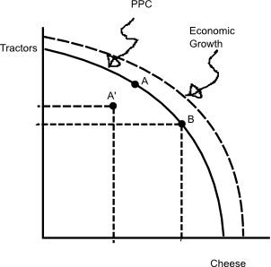
Also Production Possibility Frontier (PPF). Graph showing the production of products at maximum resource use for
all values of production.
Assumptions:
- The economy is operating at full employment and achieving productive efficiency.
- Fixed resources, ie: no big tractor parts deposits are found
- Fixed technology, ie: no major breakthroughs in cheese mold DNA construction implemented
- Two products only: a capital good (tractors) and a consumer good (CR) (cheese)
Points inside the curve (A') illustrate unemployment or productive inefficiency (compare with productive efficiency).
The difference between these points (A') and points on the PPC (eg: A) are known as the GDP gap.
Economic growth can be illustrated by an outward shift in the PPC (toward the North-east)
In general, economic growth is greater when more of the goods for the future are produced, rather
than those that are immediately consumed. In the PPC graph, if a country was producing higher on
the PPC curve (ie: a lot of tractors and not much cheese) economic growth would be faster than one
producing at a point lower on the PPC curve (ie: more cheese, not many tractors). This is because
the goods for the future allow production to be increased faster, rather than being devoted to
immediate needs.
- Law of increasing opportunity cost
-
The PPC is bowed out (concave) because the assumption is that the resources used to produce tractors and cheese are
adaptable to one or the other, but there are resources that are optimised for one or the other. Thus at maximum tractor manufacture
(no cheese production at all), only a slight drop in tractor production results in a relatively large increase in cheese production,
because those resources that are most optimal for cheese production (and least optimised for tractor production) is switched over to
cheese. As more cheese is brought on line, the slope of the PPC becomes more negative, indicating that the relatively more
tractor-optimal resources are being converted to cheese production. There is some lack of flexibility
or interchangeability that causes the marginal opportunity cost to fluctuate. If this was not the case,
the PPC graph would be a straight line.
- Efficiency, full employment and economic growth/technological improvement
-
Economic efficiency is when society gets the maximum output from its scarce resources. This requires
that full employment and full production are achieved.
- Full employment
-
All available resources are employed. "Available" can have a cultural interpretation. For example, in Australia people over the age of 65 are not required to work, so they are not included in full employment.
The production of stuff sits somewhere on the PPC
.
- Full production
-
The maximum amount of goods and service that can be produced from the
employed resources of an economy.
Involves two kinds of efficiency: 1. allocative
efficiency which occurs when all available resources are devoted to the
combination of goods most wanted by society
, and 2. productive
efficiency which occurs when goods or services are produced using the lowest
cost production methods.
Marginal cost is equal to the marginal benefit.
- Allocative efficiency
-
Occurs when all available resources are devoted to the combination of goods most wanted by society.
In other words, utility is at a
maximum.
At this point, P = MR = MC (specifically, P = MC). Explained this way: if P > MC, society favours more of the product than other substitutes, and vice versa.
- Productive efficiency
-
Occurs when goods or services are produced
using the lowest cost production methods.
ie: when ATC is at its minimum.
Productive efficiency occurs at the point where P = ATCmin.
Points along the production possibilities curve are productively efficient.
- X-inefficiency
-
The failure to produce any given output at the lowest average (and total) cost possible.
Monopolies and oligopolies are susceptible to this, due to the lack of competitive pressure.
Examples: Lack of competition may not force a firm to change to the latest technology, firm may have other goals other than minimising costs (expansion, social cohesion, avoidance of risk), may employ incompetent labour, may have non-motivated labour, may be relying on "rules of thumb" rather than thorough economic analysis to make decisions.
- Dynamic efficiency
The ability to develop the most efficient production techniques over time.
This is stuff like, developing new and more efficient technology, developing new products, anything that allows a firm to lower their average total costs. Research. Where an economy responds adequately (speedily and with flexibility) over time to change in demand and supply conditions.
That is, if there are any changes to demand (say, price drop of a substitute) or supply (say, better technology developed), the firm has the ability to respond to the change in a timely manner.
- Economic systems
-
Economies differ on two grounds:
- Ownership of means of production
- How economic activity is coordinated
- Capitalism
-
Pure capitalism is where the choice of what to produce, how much to produce is decided by the
market. Individuals own the means of production and are profit-motivated when they decide what
to produce.
Also known as a market economy
- Command economies
-
Economies where the economic decisions are decided not by the market or individuals, but by
governments. For example, China, communist Russia. Individuals do not own the means of production.
- Mixed economies
-
A little bit of capitalism, a little bit of command. Most countries are this. Sweden apparently
is a typical case of this, although the lecturer describes them as unusual.
- Authoritarian capitalism
-
A regime with a high degree of government
control with privately owned property.
- Market socialism
-
Public ownership of property, with markets
playing a significant role
- Traditional economy
-
In the traditional or customary economies found in many less developed countries, production
methods, exchange and the distribution of income are all sanctioned by custom.
Market
... any institutional structure or "mechanism" that links potential
buyers (or demanders) (D) with potential sellers (S)
. They
determine the price and quantity of a good or service transacted in a perfectly competitive market.
Types of goods
- Normal goods: Commodities whose demand varies
directly with money income, also known as superior goods.
Most goods are normal goods.
- Inferior goods: Commodities whose demand varies
with the inverse of money income. An example could be
beer. As income rises, you may stop buying beer and go for the classy stuff, like whiskey, wine etc.
- Substitute goods: Goods that can be used in place of another good;
there is a direct relationship between the price of one good and the demand for another. One example
is beer and wine. An increase in wine price may see you substituting your wine for beer, so the
amount of beer that you buy increases, and the amount of wine you buy decreases.
- Complementary goods: Goods that are used in conjunction with
each other; there is an indirect relationship between the price of one good and the demand of
another. One example is say, bread and peanut butter. If the price of bread rises, you
may not buy as much peanut butter.
- Independent goods: Goods that are not
related at all, so that a change in the price of one good will have negligible impact on the demand for the other.
- Demerit goods: Not sure if this is covered in our course - this only mentioned so far in Lecture 3. Doesn't appear in text book. Goods that the government think that are bad for society, eg: cigarettes, alcohol, and (according to the lecturer) petrol. These attract excise.
Law of Demand
The analysis of demand in this section depends on the assumption of pure competition.
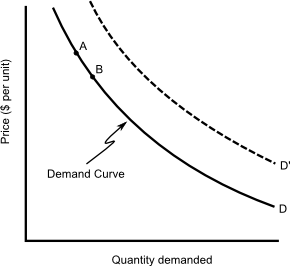
... the inverse relationship between the price and the quantity demanded of a good
or service during some period of time.
That is, P ∝ 1/Q
Demand is the quantity (Q) of a good or service that is willingly purchased at a given price (P) per
unit of time, holding all other factors constant.
The quantity (Q) demanded is dependant on price (P). That is, we can control the price, but we can't
control the quantity sold. That is, we set the quantity by setting the price. So price is the independent variable
and goes on the vertical axis (unlike mathematics, which the independent variable goes on the x axis),
and the demand is the dependant variable, which goes on the horizontal
axis.
Three things lead us to conclude an inverse relationship between demand and price:
- Observable behaviour: people do buy more products when things are cheaper
- The law of diminishing marginal utility
- Changes in prices that produce an income effect and substitution effect.
Factors affecting demand (D):
- Price
- Tastes and preferences: influenced by advertising, fashion etc.
- Expectations of future price movements (ie: if people believe prices will be going up,
they will buy more of a product)
- Personal future, ie: if you think things are going well for you, you are more confident
about making purchases. Related to above.
- Income (Y), or personal disposable income (PDI).
- Prices of other complementary goods (ie: If you buy a car, you will be buying petrol),
Prices of substitutes
- Number of buyers (D), and demographics of target market.
So, cet.par. all factors except 1. price assumed constant in our look
at price vs demand.
Factors 2-7 are non-price determinants
Note: a change in price does not change the demand curve. It indicates movement
along the demand curve, for example moving from A to B. That is, the demand (D) is the curve, and
a changing price does not change the curve, but changes the quantity demanded. That is,
a change in price does not change demand, but changes the amount demanded.
"Change in demand" means that the demand curve slides up or down along the x axis and it is
caused by a change in the non-price determinants, whereas "Change
in demand quantity" is caused by a price change (cet.par.) and is a movement along a stable demand curve.
There are two effects that are relevant:
- Income effect: ... the impact of a change in the price of
a product on a consumer's real income (purchasing power), and the consequent impact on the
quantity demanded of that product. A cheaper price means that we can buy more of a
product without reducing our spend on other products. A lower price increases our purchasing
power, and vice versa. For example, if lamb becomes cheaper, we may buy one kilo rather than half a kilo.
- Substitution effect:... the impact of a change in the
price of a product on its relative expense, and the consequent impact on the quantity demanded.
In other words, a cheaper price will encourage us to substitute the product for a similar one
that is relatively more expensive. For example, if lamb becomes cheaper, we will usually buy
more of it and less of the relatively expensive beef/pork/chook.
Diminishing marginal utility: Buying successive units decreases the utility that a product gives.
For example, one hamburger is great, two are good, but 17 is getting ridiculous. Therefore,
Consumers buy additional units only if price is reduced.
Law of demand based on:
- Demand Schedule
-
A table where the first column is the price per unit, and subsequent columns are the quantities
demanded by buyer A, B, C, ...
| Price per unit | Buyer A demands | Buyer B demands | Buyer C demands | ... |
|---|
| 4 | 10 | 12 | 8 | ... |
| 3 | 20 | 23 | 17 | ... |
| 2 | 35 | 39 | 26 | ... |
| 1 | 55 | 60 | 39 | ... |
- Demand Curve
-
Price (vertical axis) versus quantity demanded (horizontal axis).
- Individual & Market Demand
-
- Individual demand is the demand for a product of one consumer.
- Market demand is the sum of demands from a group of individuals.
- Price Change Determinant (demand)
- Non Price Change Determinant
-
- Tastes or preferences: Influenced by advertising, fashion, information.
For example, adverising Carlton Draught will cause more people to prefer it. Princess Mary holding
a Carlton Draught will increase consumers' tastes. Information on the effects of alcohol will likely decrease consumers' tastes.
the most important non-price determinant
- Number of consumers: Migration, changing demographics, population
growth, changes in transport/communication, a major outbreak of cooties. An increase shifts the demand curve to the right, a decrease
shifts it to the left.
- Money incomes of consumers: Changes in money income are a bit
more complicated in their affect on demand. It depends on the type of goods that are affected
when income changes. This usually means changes to someone's PDI.
- Prices of related goods: Related goods are substitutes and
complements. For example, we can substitute lamb for beef, and petrol is a complement to a
car.
- Consumer expectations: If you're a bit worried about
losing your job in the future, you would be reluctant to spend more than you had to. On the
other hand, if the future looked good, you would be prepared to spend more. Similar with price:
if you expect the price to go up, you will buy more product, and vice versa.
These determine the position of the demand curve. Changes in the non-price determinants
shift the demand curve along the x-axis (dependent axis). Note, it is a horizontal shift. For example, an increase in income will shift
the curve to the right from D to D' above, and an increase in taxation that lowers your PDI will shift the
curve to the left, from D' to D.
The demand (demand curve) will shift to the left if there is:
- decreased taste for product X
- decreased number of consumers in the market.
- a fall in income if product X is a normal good.
- a rise in income if product X is an inferior good.
- decrease in price of a substitute to product X.
- increase in price of a complement to product X.
- expectations of lower prices and/or incomes.
The demand (demand curve) will shift to the right if there is:
- increased taste for product X
- increased number of consumers in the market.
- a rise in income if product X is a normal good.
- a fall in income if product X is an inferior good.
- increase in price of a substitute to product X.
- decrease in price of a complement to product X.
- expectations of higher prices and/or incomes.
- Price elasticity of demand

-
- Definition: The ratio of the relative change in quantity demanded and the relative change in price. That is:
Ed or PED = (ΔQ / Q) / (ΔP / P) = (ΔQ x P) / (ΔP x Q)
- Graphing: Generally, the price elasticity of demand on the upper portion of the curve is elastic, whereas the lower portion it is inelastic. The elasticity is not the slope of the graph. You are more likely to change your consumption habits if price of an expensive thing changes by 1% than you would if something cheap changes price by 1%. For example, a 1% change in the price of a house which may be of the order of $3000 is of far more significance to you than a 1% change in price of chewing gum, which may be $0.03. What's an extra 3 cents? Nuthin', I'll buy it anyway, but an extra $3000 for a house? That's plenty, so I'm more likely to not buy a house.
- Measurement & calculations:
- Midpoint: In the above demand graph, to calculate the elasticity of going from A to B, calculate the elasticity at the midpoint. That is
ΔPmidpoint = ΔP = PB - PA
and Pmidpoint = (PA + PB) / 2
and ΔQmidpoint = ΔQ = QB - QA
and Qmidpoint = (QA + QB) / 2
Ends up being:(ΔQ x (PB + PA)) / (ΔP x (QB + QA))
- Total revenue method: Graph the total revenue (TR) versus the quantity demanded.
TR = P x Q
At the peak, E = 1. A "positive" slope means E > 1 (elasticity), whereas a "negative" slope means E < 1 (inelasticity).
- Determinants:
- Substitution:
Generally, the larger the number of good substitute products available, the greater the elasticity of demand.
For example, an increase in the price of VB will have consumers changing to Tooheys and Boag. Also, the closer the substitution, the more the effect.
- Proportion of income: Cet.par.,
the higher the price of a good relative to your budget, the greater will be the elasticity of demand
. For example, a 10% rise in car prices will drop demand for cars quicker than a 10% rise in chewing gum would drop demand for chewing gum.
- Luxuries versus necessities: Luxuries tend to be elastic, whereas necessities tend to be inelastic. For example, you don't have to buy a Porsche to survive, so when times are tough, you forego Porches for second-hand cars. But if you're diabetic and you need your insulin to survive, you will buy it no matter what the cost.
- Time: (Δtaste?)
In general, the longer the period under consideration, the more elastic is the demand.
People are creatures of habit. They will take time to change their product over as they train their preferences over to the other product. For example, an increase in price of wine may push more people over to preferring beer over time, as they change their preferences and get used to the other product.
- Summary
-
Taken from JI Table 6.2 p 159. Note: do not assume the slope of the demand curve is an indicator of the elasticity!
| Value of Ed | Terminology | Description | Impact on Total Revenue |
|---|
| Price Increase | Price Decrease |
|---|
| Ed = ∞ | Infinitely or perfectly elastic | Quantity changes maximally for an infinitesimal price change (demand curve is horizontal) | TR = 0 | TR = ∞ |
| Ed > 1 | "Elastic" or "Relatively elastic" | Quantity demanded changes by a larger percentage than price (demand curve will be "flat-ish") | TR ↓ | TR ↑ |
| Ed = 1 | "Unit" or "Unitary elastic" | Quantity demanded changes by the same percentage as price | TR unchanged | TR unchanged |
| Ed < 1 | "Inelastic" or "Relatively inelastic" | Quantity demanded changes by a smaller percentage than price | TR ↑ | TR ↓ |
| Ed = 0 | Perfectly or infinitely inelastic | No change in quantity for any change in price (demand curve is vertical) | TR ↑ | TR ↓ |
Note that marginal revenue (MR) is positive when demand is elastic, zero when demand is unitary elastic, and negative when demand is inelastic.
Law of Supply
The analysis of supply in this section depends on the assumption of pure competition.
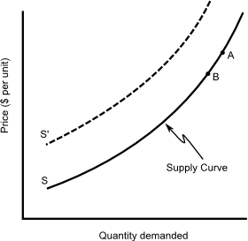
The quantity of a good or service that produces will willingly supply at a given price per
unit time assuming cet.par. That is, P ∝ Q
Positive relationship can be explained in two ways:
- Rising prices are an incentive to supply more stuff and vice versa.
In other words, if suppliers are making a lot of cash, then they will do their best to increase
production to bring in even more cash. They will strike while the iron is hot, so to say.
Increases in production often cause rises in the price of certain inputs, particularly
those whose supply cannot be readily increased, such as specialised labour and raw materials.
There are also some factors of production, such as the factory, plant and equipment, that cannot be expanded in response to increased production.
At some point, these fixed factors of production become
over-used and the lower productive efficiency of these fixed factors of production increases
the per-unit cost of production. As a result, producers need a higher price to compensate
them for the higher costs that are associated with greater production.
A farmer who grows mixed crops will generally (cet. par., assuming the other
crops don't rise as well) put the more resources into growing the crop that he gets the best
price for, and therefore as prices increase, supply increases.
A manufacturer will only be able to supply so much product. As prices increase, he uses the
extra revenue gained to increase the production capacity of his plant, to maximise profit.
Similarly to demand, a "change in supply" means a change in one or
more of the non price determinants, shifting the curve left or right along the x-axis. A "change
to supply quantity" is caused by a change of price (cet.par.), and is a movement along a stable supply curve,
say A to B.
Supply curve based on:
- Common sense and observation
- Price as revenue per unit and an incentive to produce and sell a product
- Rising costs and declining productive efficiency
- Supply Schedule
-
Similarly to demand schedule, a table showing the quantity of product supplied at each
price point.
| Price per unit | Supplier 1 | Supplier 2 | Supplier 3 | .... |
|---|
| 5 | 60 | 70 | 40 | ... |
| 4 | 49 | 50 | 38 | ... |
| 3 | 38 | 32 | 35 | ... |
| 2 | 27 | 17 | 31 | ... |
| 1 | 16 | 4 | 26 | ... |
- Supply Curve
-
The supply curve is the graph of price per unit versus quantity supplied.
- Price Change Determinant (supply)
- Non Price Change Determinant
-
- Production costs: Costs of N, L, K (cost of factors of production).
Costs of resources. An increase in resource prices shifts the supply
curve to the left, and vice versa. This can be explained that the "price" is bound
up in revenue for the company, therefore there is less incentive to produce more. Consider
the farmer example above. If the price of wheat seed goes up, then the wheat isn't so attractive
to plant, and he may devote land to other crops instead.
- Technology: This is a decrease in the cost of capital, an increase in production efficiency, and hence would shift the supply
curve to the right. It may also result in the ability to use fewer resources for production, or
use the current resources to produce more product.
- Prices of other goods: for our farming example, a decrease in the price of wheat may mean that
the farmer will increase production of another crop, to maximise his return.
- Expectations: A complex issue. If the price of wheat goes up, our farmer may withhold some
wheat in the expectation of being able to sell it at a higher price later, causing a decrease
in the amount of wheat produced. Other farmers may increase their wheat acreage, in anticipation
of those increases. Depends on a case-by-case thingo. Depends on the ability of companies to
alter production or store products.
- Number of sellers in the market: More sellers means the curve shifts to the right, less to the left.
Extra ones that the lecturer tacked on:
- Productivity: This could be seen as a decrease in the cost of the labour (L) resource, therefore
similar to the above point.
- Climatic factors
The supply curve will shift to the left when there is:
- an increase in resource prices.
- increased prices of other goods they produce
- expectations of future prices (usually)
- decreased number of sellers
The supply curve will shift to the right when there is:
- a decrease in resource prices.
- improved production technology
- decreased prices of other goods they produce
- expectations of future prices (sometimes)
- increased number of sellers
- Price elasticity of supply
-

- Definition: Price elasticity of supply depends on what time frame you look at. The time frames are:
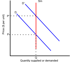 Market period or Immediate period: This is the period immediately after a price change (P to P'). The producers have no chance to make any changes to adjust the quantity supplied to the new price, so it stays at Q. An example: a producer brings a truck-load of tomatoes to the farmers' market. Because demand is high, he sells the lot, however he can't produce more there and then to satisfy demand. The truck-load is all he's got for now. Price elasticity of supply is almost perfectly inelastic.
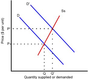 Short run: In the short-run, the producers are starting to change their production to suit the new demand. At least one, but not all of their inputs have changed to meet the increased demand. Cet. par. equilibrium price will drop slightly, equilibrium quantity will increase slightly. For our tomato farmer, he may buy some more or better fertiliser for his tomatoes, change his crop allocation to more tomatoes, etc.
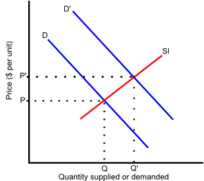 Long run: Suppliers have had all the time they need to adjust to the new level of demand. Producers have done what they can to meet the new demand. Cet. par. equilibrium price will drop more, equilibrium quantity will increase more. Our tomato farmer has bought more land for tomatoes, new tomato farmers have come into the business etc.
- Graphing:
- Measurement & calculations:
- Determinants:
- Time: Market period, short-run and long-term. This is the primary determinant.
- Nature of good: Is it durable or perishable? Perishable implies a low PES (inelastic).
Equilibrium, or Market Equilibrium
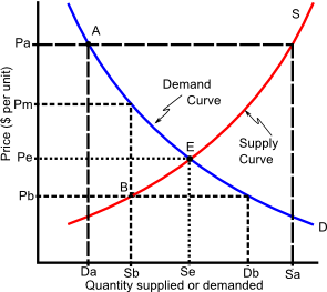
Equilibrating process: Market forces that push prices towards equilibrium.
For example, if the price Pb is below PE, then the amount that producers willingly supply is less than the
amount that consumers willingly want to buy, therefore it is a shortage of Db - Sb units, buyers compete to buy the product, pushing up the price towards equilibrium.
If the price Pa is above PE, then there is a surplus of (Sa - Da) units. The quantity producers
willingly supply is more than what consumers are willing to buy, producers discount stock to sell and that pushes the price down towards equilibrium.
Markets discover prices.
Market is at point E, the intersection of the supply and demand curves, in state of balance, there are no shortages and no surpluses.
Quantity supplied equals quantity demanded (Se = De), being sold at the equilibrium price (Pe). This is the equilibrium quantity.
The equilibrium price (Pe) is also called the market-clearing price
because it clears the market, leaving no inconvenient surplus for the sellers and no
inconvenient shortage for the potential buyers
, or everything that is offered for sale
is sold
.
The ability for a market to push towards equilibrium is sometimes called the rationing function
of prices. It is the market forces "rationing out" resources and products to the buyers who
are willing and able to purchase them.
Surplus & Shortage
A surplus or excess supply (A) happens when the product price (Pa) is above the equilibrium price (P e).
Suppliers have the incentive to produce more (Sa) than what the consumers are demanding (Da),
producing a surplus of (Sa - Da) units. Competition between producers causes the
price to push towards equilibrium.
A shortage or excess demand (B) happens when the product price (Pb) is below
the equilibrium price (Pe). Suppliers have little incentive to produce (Sb), and
consumers are frothing at the mouth to buy (Db), producing a shortage of (Db - Sb) units.
Competition between buyers forces up the price toward equilibrium.
Sometimes the shortages and surpluses are artificially produced. Such as:
- Minimum prices: AKA price floors (Pa). Causes surpluses. For example, government says a price must be a minimum, usually to protect producers. Happened in the wool industry producing an oversupply of wool. Government bought excess, then had to advertise to change consumer tastes to increase demand to get rid of excess stocks. Producers then were competing against the government wool stocks for market, so they reduced the number of sheep. Another example: unions enforcing minimum wage rates, produces an oversupply of labour.
- Maximum prices: Also known as price ceilings (Pb). Causes shortages. One rationale is to protect consumers. One method that governments deal with shortage is to impose rationing, like they did in WWII, that is people are only allowed to buy so much butter etc. This produces black markets, where some consumers are prepared to pay much higher prices for the product, up to Pm.
Unpredictable and predicable cases of price and output
Single shifts in parameters
| Change | Price | Quantity |
|---|
| D↑ | P↑ | Q↑ |
| D↓ | P↓ | Q↓ |
| S↑ | P↓ | Q↑ |
| S↓ | P↑ | Q↓ |
Effects of changes in S & D on P & Q
| Supply | Demand |
|---|
| Increases | Steady | Decreases |
|---|
| Increases | P? Q↑ | P↓ Q↑ | P↓ Q? |
|---|
| Steady | P↑ Q↑ | - - | P↓ Q↓ |
|---|
| Decreases | P↑ Q? | P↑ Q↓ | P? Q↓ |
|---|
Those marked with a "?" above: The amount and direction of the change depends on the comparative scales (magnitudes) in ΔS & ΔD. Terminology is that whatever is indeterminate.
Guiding function
Part of the price mechanism. Producers are guided by price into allocating resources (N, L, K) to produce products. For example, 1995: Australian wines won some prestigious gold medals. Global demand went up, so farmers started changing crops to wine grapes.
Market Structures or Market Models
- Profits & production
-
For all businesses, profit maximization or profit maximization rule happens when MC = MR. Logic behind this: if MR > MC, ie: total revenue is rising faster than costs, it makes sense to increase production to capture more revenue hence more profit. However if MR < MC, ie: total costs are rising faster than total revenue, it would make sense to reduce production volumes to increase your total revenue.
Profit maximization can be stated another way: profit is at a maximum when TR - TC is at a maximum, ie: when the difference between the total revenue and the total cost is at its maximum.
The points where the TR curve cross the TC curve are the break-even points. The break-even point is where the MC curve cuts the ATC curve.
How does a firm know when and how much to produce? Three different scenarios:
- Part of the TR curve lies above the TC curve: The profit-maximizing rule above holds, and the firm should produce at the quantity where
MR = MC, making an economic profit.
- All of the TR curve lies below the TC curve, but part of the TR curve lies above the TVC curve: The firm should produce at the loss-minimising point, ie: where
TR - TC < TFC. ATCmin > P > AVCmin. There will be some level of production that will achieve the minimum loss. At that point, the total revenue will be covering all the firm's total variable cost, with some extra to off-set some, but not all, of the firm's fixed costs. At this point, MR = MC, but . The minimum price-point that this is going to happen is when price equals the minimum average variable cost, P = AVCmin. This price is known as the shutdown point or close-down point.The difference at this point compared to the profitable company is that marginal costs are falling at this point, ie: the slope of the MC curve is negative
- All of the TR curve lies below the TVC curve: This is the close-down case. The firm in the short-term, should shut down. Any level of production will increase losses. The firm's losses are equal to its fixed costs. The price is below the minimum average variable cost (
P < AVCmin). The close-down point is where the MC curve cuts the AVC curve.
Except for pure competition, marginal revenue is always greater than price MR > P.
A firm should produce if it either can make a profit, or make a loss less than it's fixed costs. Just to explain that second point: Whether a firm is producing or not, it is incurring its total fixed costs (FC). If there is no point at which the firm is making a profit, then there may be a production point where the firm is making a loss that is less than the total fixed cost. That is, if a firm's fixed cost is $100 per month, there might be no production volume that will make a profit, but say at the point of production of minimum loss it may only be losing $70. So the firm will only be losing $70 if it produces, rather than $100.
If MC < MR (= P), this is underallocation, means that adding more units will increase profits. Another way of saying this is that society values additional units of this product rather than any substitutes they can buy.
if MC > MR (= P), this is overallocation, and means that production should be cut to increase profits. Saying this another way is that society values the substitutes more than this product.
Taken from JI Table 10.7 p 283
| | TR TC approach | MR MC approach |
|---|
| Should the firm produce? | Yes, if TR > TC or if 0 < TC - TR < TFC | Yes if P ≥ AVCmin |
|---|
| What quantity should be produced to maximise profits? | Either TR - TC is maximum, or (TC - TR)min < TFC | MR = MC and MC↑ |
|---|
| Will production result in Π > 0? | Yes if TR > TC, no if TR < TC | Yes if P > ATC, no otherwise |
|---|
Information on the different markets can be broken up into three sections: 1. Structure; 2. Conduct; and 3. Performance.
- Pure Competition
-
Also perfectly competitive market, and perfect competition.
- Products are homogeneous (see note below).
- Many small firms.
- Individual producers have negligible production volumes compared to the market volume hence have no significant influence on price, hence are price takers (as opposed to price makers, who have the influence to set prices). However, the all producers acting at once can influence price. For example, all producers can drop production by 5%, cet. par. increasing the price.
- Producers are free to enter and exit the market, that is
there are no legal, financial or technical barriers to market entry.
- No non-price competition (eg: advertising, brand differentiation, quality differentiation, sales etc)
Not realistic. No good real-life examples. More an abstraction for comparison purposes. Closest real-life examples probably would be some agricultural products, wool industry.
Homogeneity of the products means that from the individual firm's point of view, the product has perfect elasticity of demand (ie: the demand curve is horizontal) due to its perfect substitutability. Because of homogeneity, consumers can buy it from any firm. Implies consumers' perfect knowledge?
Note that the market demand curve (the sum of all the individual firms' demand curves) looks like what a normal demand curve would look like (going from top left to bottom right, straight or curved line).
Revenue concepts:
TR = P x Q Price is constant over the range, so the only adjustment a firm can make is to quantity produced. Therefore, graphically, the TR line is a straight line.AR = TR / Q = P That is, the average revenue is the price assuming there are no taxes on the product, because the firm, being a price-taker, can't control the price no matter what volume it produces.MR = ΔTR / ΔQ = (ΔQ x P) / ΔQ = P, ie: Rate of change (slope) of the TR curve. Price is a constant, therefore marginal revenue is constant and is equal to price.- Uniquely in this market model for a firm producing at the profit-maximising point,
AR = P = MR = MC, ie: Π = TR - TC = 0, ie: the firm is making zero economic profit, ie: the firm is making normal profits only.
- Lack of economic profit makes it hard for a firm to have dynamic efficiency, due to competitors quickly implementing or imitating any new technology changes.
All the above assumes that there are no taxes imposed on the product. If taxes were imposed, AR would not equal Price.
Above the close-down point, the individual firm's marginal cost curve is its supply curve.
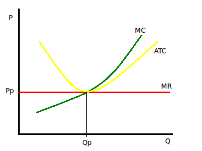
Long-run assumptions:
- The only thing of significance is the entry and exit of firms into and out of the industry.
- All firms are assumed to have similar cost curves.
- Entry and exit of firms does not affect resource prices, ie: constant costs. An increase in demand will initially put the price up producing an economic profit for the firms in the industry, more firms are then attracted to come into the market, price falls back to what it was, and firms are back to making only normal profits. In the assumption of constant costs, the long-term supply curve for the industry is horizontal.
- Entry and exit of firms push towards all firms making only normal profits, that is, zero economic profit.
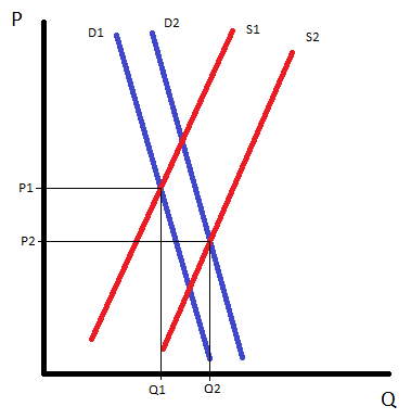
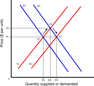
Explanation of the reaction to increasing demand in a constant-cost purely competitive market: (Refer to "Reaction to changing demand ..." figure.) Initially, the supply and demand curves are S1 and D1, producing an equilibrium price of Pc at a production level of Q1, at point e1. All firms in the industry are making normal profit only, ie: zero economic profit. An increase in demand (curve D2) initially causes a change in the quantity supplied, ie: a movement up the S1 curve to the point e2. The buyers have competed the price up to P2. At this point, the firms are making an economic profit, and this attracts more firms into the industry, eventually increasing the supply to curve S2. The extra firms compete away the economic profit, and bring the equilibrium down to point e3, at which point all firms are again only making normal profits.
Three different scenarios for industry supply in the long-term:
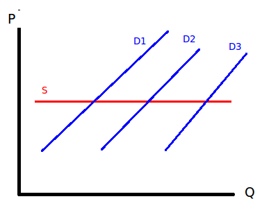 Constant cost: As above. Entry/exit of firms does not affect resource prices. The long-term industry supply curve is horizontal to the Q axis. That is, supply is perfectly elastic.
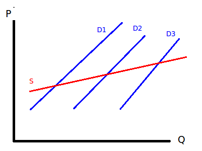 Increasing cost: Entry into the market causes the resource costs to increase, as firms bid-up the price. The long -term industry supply curve has a positive slope.
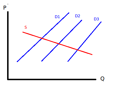 Decreasing cost: Apparently this does happen. One example: mines open up in an area. The first mine to open up has to use relatively more expensive transport to get their ore to market. As more mines open up in the area, it may become convenient to put in a rail line, decreasing transport costs. In this case, the long-term industry supply curve has a negative slope.
Efficiency:
- Productive efficiency: (See definition) Producing at the minimum of the average cost curve.
- Allocative efficiency: (See definition) Implies that
P = MC.
- Pure Monopoly
-

See also a natural monopoly.
One company provides the service or good. No really good examples in real life. Economists believe that monopolies don't last forever. Market forces too strong for monopolies to exist in the long term.
Textbook monopolies are (for the current time period under consideration):
- One firm only.
- Price makers: ie: they can set the combination of P and Q to produce. They can decide where on the demand curve to produce their product. One implication of being a price-maker in real-life: firms don't necessarily have to set their production point at the point of profit-maximisation. They can choose other points for other reasons.
- No immediate rivals and no close substitutes.
- There are barriers to entry, or blockaded entry, so that the firm is protected from other firms coming into the market, ie: new firms coming in will have higher costs initially. Barrier could be real or perceived.
- As with all firms, we assume the goal of the firm is to maximise profits (however, see note in the "price-makers" dot point above).
Monopoly model assumptions:
- Monopolist's position guaranteed by barriers to entry
- No possibility of government take-over, or being restricted by government regulation
- Single-price monopolist, and that all product is sold.
Revenue concepts:
- Unlike the firm in a purely competitive market, a monopoly's demand curve is the market demand curve.
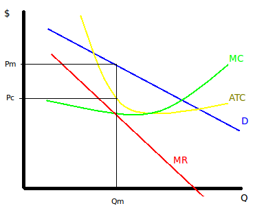
A monopolist doesn't really have a supply curve. If it is a single-price profit-maximising monopolist, there is only one point on the demand curve it will produce at, the profit-maximising point MC = MR.
If the supply curve is required, the marginal cost curve will be the supply curve.
Demand curve of the monopolist is the average revenue curve.
- Being a price maker, it can charge any price it likes, but has to take the resultant demand quantity. Or it can produce a certain amount, but it has to accept the price for that quantity. That is, it can control price or quantity, but not both. On prices, it can choose to be a:
- Single-price monopoly: one price for all and sundry;
- Price-discriminating monopoly: charging different prices to different categories of buyers despite the same production cost, eg: student discounts.
- Firm assumed to face same costs as a firm in pure competition, so it's cost curve looks the same.
- Marginal revenue is not the same as price, because of the downward-sloping demand curve (except, of course, for the very first item produced). MR is dropping after the first unit, because the monopoly is supplying the market, and the market demand price drops for each additional unit produced for all units produced, not just the marginal unit.
P > MR. As MR is dropping, this implies AR > MR, as AR = P assuming no taxes.
- Profit-maximising at
MR = MC. As MC is always positive, the profit-maximising point will be somewhere in the elastic part of the demand curve.
- Because
P > MC, allocative efficiency is not achieved.
- Because
P > ATC, productive efficiency isn't achieved.
- Susceptible to X-inefficiency due to lack of competitive pressure.
- Because of the ability to produce an economic profit, monopolies are able to have dynamic efficiency, however there may be a lack of incentive to do so due to lack of competitive pressure. Countering that, there is an increased profit to be had in dynamic efficiency, and this may motivate the monopolist to chase this. In other words, a monopolist has the choice to be dynamically efficient or not.
The demand is elastic where the marginal revenue is positive. At the point where marginal revenue is zero, the elasticity of demand is unitary. Where the marginal revenue drops below zero, the demand is inelastic.
Short-run and long-run situations for a monopoly are identical. This is because there are no rivals to compete with to share the profit around. That means that any economic profit is maintained, and there is no market pressure to force movement to normal profit only.
Monopolies created by:
- Barriers to entry: (see dot-point above). Examples:
- Legal: patents, government-supplied licences, copyright laws;
- Natural or exogenous factors: economies of scale (see natural monopoly), product differentiation, control of an essential input (eg: China owns most of the rare-earth production therefore can legislate to reduce exports, handing Chinese companies a "monopoly" on industries that use rare-earth elements as an input). A monopoly experiencing economies of scale may mean that a firm coming into the market may have to spend the money for a large plant just to be able to compete with the monopolist.
- Sunk costs: start-up costs that you don't get back, such as schmoozing the retailers to start stocking your product, heavy initial advertising, paying government licensing fees etc;
- Strategic barriers: A firm choosing to act to protect its operating environment from rivals. Examples: threats, advertising, vertical integration (controlling resources or retail), predatory pricing (pricing below cost or price-matching), raising rival's costs, dirty tricks etc. Not necessarily illegal or morally ambiguous stuff.
- Spatial factors: eg: geographic isolation, perishable products, high transport costs.
- Temporal factors: transient stuff - here today, gone tomorrow. Example: rock concerts.
Myths about monopolies:
- Monopolies are big: Not necessarily. A monopoly means just an absence of rival firms. The only chemist in a small town has a geographic monopoly.
- Big is bad: Not necessarily. Big firms can afford to to expensive R & D.
- Monopolists can charge what they like and/or do what they like: No, restrained by what the market will accept.
- Monopolists maximise profits: Usually, yes, but there are other goals. Examples: sales maximisation - goal is to be the biggest; Stakeholder satisfaction - goal is to keep workers, customers, unions etc happy
- Monopolies are durable: No. Long-term, other firms can come into a market, overcoming the barriers. Market forces will prevail. Innovation, technology change. Only monopolies that endure are government-backed ones, eg: Australia Post.
- Monopolists never make losses: Usually yes, but depends on where the cost curves and market demand curves are. Demand can shift due to changing tastes etc.
- Monopolists subject to higher costs because of the lack of market pressure: Some evidence of some firms allowing costs to drift up, but usually countered by the benefits of economies of scale.
- Monopolies restrict output compared to purely competitive firms: That is, compared to a pure competition scenario, the output levels are further to the left on the demand curve. Probably true. True for single-price monopolists, untrue for price-discriminating monopolists.
PM > PPC and QM < QPC. Economists argue that monopolies are allocatively inefficient, because the profit-maximising point sits away from the equilibrium. The difference between the profit-maximising point and the equilibrium is called the dead weight loss.
Market forces / government regulation bring real-life monopolies into check. Patent conflicts can be avoided by engineering a different method or product that substitutes for the monopolist's product.
Price discrimination
Price discrimination: When a firm charges different customers a different price for the same good when the costs of supply are identical
, for example: MS Office student discount, student discount on public transport. Or When a firm charges different customers the same price for the good when the costs of supply differ
, for example: health insurance - married couples pay same rate as singles. Or when a given product is sold at more than one price and the price differences are not justified by cost differences.
Only done by a firm with market power, with knowledge of the demand elasticities of different buyers (ie: a segmented market) at different prices, and are able to prevent resale between buyers. Not all price differences for the same good are price discrimination. They may reflect real differences in the cost of supply. Monopolists price-discriminate to increase profits by increasing volumes. Three main types of price discrimination:
- First degree: haggle/negotiate a price. Examples: auctions, street markets, illegal goods, used car dealers (don't reveal your reservation price! When they ask you "What's your budget?", say "Enough for a second-hand whatever-car-you're-after"). Can be allocatively efficient similar to a perfectly competitive firm, because quantities are not restricted. Unlike a perfectly competitive firm, a first-degree monopolist will get maximum return for all quantities. Eg: Sell first unit to highest bidder, second unit to second highest bidder etc. Compare this with a purely competitive firm: All units sold are sold at the market price.
- Second degree: Volume or step-pricing. Paying less per unit for bulk purchases. Paying less for extra large size. Two-for-one deals.
- Third degree: Also multi-market pricing. Group discounts (families, students, clubs etc). Profit-maximising price will be highest in the group that has the lowest elasticity of demand. Temporal discounts (opening nights, high price for early adopters, hard-cover versus soft-cover (hard-covers come out first, but are not much dearer to make), discounts for locals (locals know the area, can choose other stuff), the Entertainment Card, electricity cheaper for industrial use than domestic, etc).
Price discrimination allows a monopolist to usually produce a larger volume of product, and increase profits.
Graphically, the perfect price-discriminating monopolist's marginal revenue curve would be the demand curve. In this case, the monopolist would be able to sell the first unit produced to the person who can and does pay the most, the next unit to the next-highest bidder and so on. Compare this to a single-price monopolist: a price is for all units produced, that is, the guy who is willing and able to pay $200 is only paying $50, the same price as the guy who is only willing and able to pay $50, whereas in a perfectly price-discriminating monopoly, the guy willing and able to pay $200 is charged $200, whereas the guy willing and able to pay only $50 is charged $50.
Regulation
Socially optimum price: the price where P = MC. That is where the demand curve crosses the marginal cost curve. This is where the price/production would be under conditions of pure competition. Unlikely for government regulation to set the price here, because the monopolist will likely be making losses, and would need permanent subsidies.
Fair return price: the price where P = ATC, ie: where the demand curve cuts the average total cost curve. In this case, the monopolist would only be making normal profits.
The dilemma of regulation occurs in choosing at which price-point is the right one to set and whether to condone price discrimination. Do we set a price closer to the socially optimum price and provide subsidies to the firm or do we set it closer or at (or above, maybe?) the fair return price?
- Monopolistic competition
-
Structure
- Many firms.
- Relatively easy entry. May be some legal (copyright/patent related), financial barriers (eg: heavy initial advertising), but not too onerous.
- Firm's demand curve is downward sloping because of differentiation, but more elastic than a monopoly due to many close substitutes.
- Limited control over prices due to product differentiation
- Small market share
- No collusion - costly to organise.
- Firms are independent, ie: no mutual interdependence like there would be in an oligopoly.
- Product differentiation.
Conduct
Product differentiation: either real (eg: different ingredients) or imagined (different packaging). Any tangible or intangible feature of a product that sets it apart from other similar products, resulting in a preference for that product among buyers.
- Product quality: physical differences, materials used, skill of manufacture
- Services: prestige of store, staff friendliness, purchasing options, training, home-delivery etc
- Location and accessibility: Milk-bar competing with supermarkets due to convenient location, a company operating 24/7 rather than the Monday to Friday 9-5.
- Promotion and packaging: Advertising, brand names, trademarks.
Plenty of non-price competition, eg: advertising, sales, levels of service,
Performance
Short run: Able to achieve economic profit in the short run.
Long run: Normal profits only, due to low barriers of entry.
- Oligopoly
-
Structure
Few large firms, each with a significant market share. Collectively, these firms dominate the market.
Basically, if your demand curve depends on what other firms in the industry does, it is an oligopoly. The situation when the number of firms in an industry is so small that each must consider the reactions of rivals in formulating its price policy
and quantity policy. That is, the firms are mutually interdependent.
Concentration ratios: The percentage of total industry sales accounted for by a given number of the largest firms in each industry.
Barriers to entry significant.
Conduct

Plenty of non-price competition.
Before a firm moves on prices, it has to predict how its rivals react to it. That usually is very uncertain. If it drops prices, will the rivals match it or undercut it, generating a price war? If it raises prices, will its rivals move with it or keep their prices the same? This uncertainty usually is a force for firms to do nothing on price. If profits are acceptable, there is usually good reasons for prices staying put (sticky pricing), because any move in price is more likely to have negative effects for the firm.
Cost-plus pricing or mark-up pricing: Oligopolist estimates the cost per unit of output, then adds a mark-up (usually a percentage of the costs) to determine price. Handy for the firm that has multiple products, due to difficulty of assigning proportions of fixed costs to each product. Can be the way a cartel sets prices.
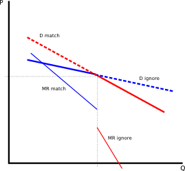
Explanation of the kinked demand curve: Oligopolists believe their demand curve to be kinked, shown as the solid lines in the figure close to here. The assumption here is that rivals will match any price drops, but not respond to any price rises, hence there are two different demand curves. That is, the rivals will keep their prices the same if the firm raises their price. The demand curve where rivals ignore (don't match) the firm's price rises (Dignore) is relatively more elastic than the demand curve where the rivals match the firm's prices (Dmatch), because where the rivals are matching prices, the difference in quantities are only due to the buyers included/excluded by the new price, and the quantity changes are shared between all the oligopolists. If the rivals don't match, then buyers then have an additional factor to consider. If the firm increases prices, buyers will change to the rival firms, hence a larger change in quantity for a certain change in price. That is, the firm loses market share to its rivals. Notice that price adjustments up or down is a "no win" situation.
The kinked demand curve shows that any movement in price is a "no win" situation. If a firm puts prices up, rivals don't follow and the firm loses market share. If a firm puts prices down, rivals will at least match it to protect their market share, and because of the relative inelasticity of the demand, a drop in price means a drop in total revenue.
Notice that for the kinked demand, the marginal revenue curve is discontinuous.
There is a great motivation for rivals to match price decreases because they must protect their market share.
Collusive oligopoly
Perfect collusion: both price rises and falls are matched by all firms in the oligopoly.
Cartels: groups of firms that agree either formally or informally to set prices and output levels of particular products among members.
Gentlemen's agreement: a form of collusion whereby groups of firms agree verbally to set prices and output levels of particular products among members
. Very hard to prove.
Price leadership: a type of gentlemen's agreement in which oligopolists automatically follow the price incentives of the dominant firm in an industry.
Price changes don't happen frequently, only when major changes to costs or demand occur. Has the risk for the leader of the other firms not following suit, if it's a price increase. Coming changes usually flagged by industry discussion in the public arena lead by the leader firm. New price may be chosen with consideration to discouraging new firms coming into the industry, so the new price may be set at less than the profit-maximising point (limit-pricing or price-blocking strategy).
Under perfect collusion, assuming identical cost and demand curves, firms in an oligopoly would set their price and quantity at the MR = MC point, ie: identical to a monopoly.
Obstacles to collusion:
- Differences in costs and demands: the profit-maximising points for the firms in the cartel may be significantly different, therefore agreement on price/quantity may be hard to achieve; compromises will have to be made.
- Number of firms: Cet. par., the more firms in the cartel, the more difficult it is to come to an agreement.
- Incentive to cheat: firms within the cartel have an incentive to cheat. Secretive price-cutting will garner more market share. Has the risk of the buyers then playing one cartel member off the other.
- Recessions: slumping markets (demand and marginal revenue curves shifting left) have the firms moving up on their average total cost curves. Profits are down, firms have excess capacity. The firms may see the need to cut prices to increase their market share and recover more profits.
- Legal obstacles: Trade practices laws.
Performance
Susceptible to X-inefficiency due to lack of competitive pressure.
Based on Table 8.1 p 222 JI
| Characteristic | Market Model |
|---|
| Perfect Competition | Monopolistic Competition | Oligopoly | Pure Monopoly |
|---|
| Number of firms | A very large number | Many | Few large firms dominate | One |
|---|
| Type of product | Standardised | Differentiated | Standardised or differentiated | Unique; no close substitutes |
|---|
| Control over price | None | Some, but within narrow limits | Constrained by mutual interdependence; considerable with collusive behaviour | Considerable |
|---|
| Entry conditions | Very easy, no obstacles | Relatively easy | Significant obstacles present | Blocked |
|---|
| Non-price competition | None | Considerable emphasis on advertising, brand names, trademarks, etc | Typically a great deal, particularly with product differentiation | Mostly public relations advertising |
|---|
| Australian examples | Agriculture (but see note above) | Retail trade; fashion | Motor cars, cigarettes, canned fish, beer | Refined sugar; steel; gas, water & electricity in some states |
|---|
Elasticity

The elasticity is not the slope of the supply/demand curve. Slopes use the absolute changes, whereas elasticity talks about relative changes. DO NOT JUDGE THE ELASTICITY BY THE SLOPE OF THE DEMAND CURVE. Generally, the upper portion of the demand curve is elastic, the lower inelastic. See here for calculated elasticity of a demand curve with a constant slope (ie: Q = a - bP)
Can be looked at as the degree of responsiveness of quantity willingly demanded to price.
Elastic demand/supply is where the per cent change in price is greater than the per cent
change in quantity demanded/supplied, that is: E > 1. Demand curve would be "flat-ish".
Inelastic demand/supply is where the per cent change in price is less than the per cent
change in quantity demanded/supplied, that is: E < 1
Unit elasticity is where the per cent change in price is equal to the percent change in quantity demanded, that is: E = 1 At unit elasticity, marginal revenue is zero, ie: MR = 0
A vertical section on a demand graph (ie: parallel to the P axis) is perfectly inelastic demand, where the quantity doesn't change no matter how much the price changes. For example, a mum who buys two school uniforms for her son each year, no matter what the price. E = 0?
A horizontal section of the demand (ie: parallel to the Q axis) is perfectly elastic demand, where an infinitesimal change in price will have the consumers going from buying nothing to buying everything they can get (perhaps where Apple releases a new product?). E = ∞?
- Price elasticity
- Income Elasticity
-

- Positive income elasticity - normal goods: The income elasticity of normal goods will be positive. That is, as income increases, people buy more stuff.
- Negative income elasticity - inferior goods: The income elasticity of inferior goods will be negative. That is, as income increases, people buy less of this kind of stuff.
- Cross price elasticity
-

- Positive cross-price elasticity - substitute goods: If the cross-price elasticity is positive, this means that products X and Y are considered substitute goods.
The larger the positive coefficient, the greater the substitutability between the two products.
- Negative cross-price elasticity - complementary goods: If the cross-price elasticity is negative, this means that products X and Y are considered complementary goods.
The larger the negative coefficient, the greater the complementarity between the two goods.
- Zero (or near zero) cross-price elasticity: If the cross-price elasticity is zero or near enough to, it means that X and Y are unrelated or independent goods. For example, a change in the price of butter will usually have a negligible effect on the demand of chewing gum.
Incidence of Tax

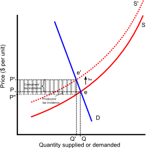
The incidence of a tax is the proportion of a tax rise or fall that consumers and producers pay.
The consumers' tax incidence is (P' - P), whereas the producers' tax incidence is (P - P'').
The tax revenue raised is TRtax = (P' - P'') x Q' (the hatched area), while the change in revenue for the producer is ΔTRproducer = (P'' x Q') - (P x Q).
In general, the more the price elasticity of demand is, the less the consumer tax incidence and greater the producer tax incidence, and vice versa.
The more inelastic the demand for a product in the relevant price range, the greater will the proportion of the tax that is shifted to consumers; the less elastic the supply, the lower the portion bourne by consumers.
Case studies
- Farming
-


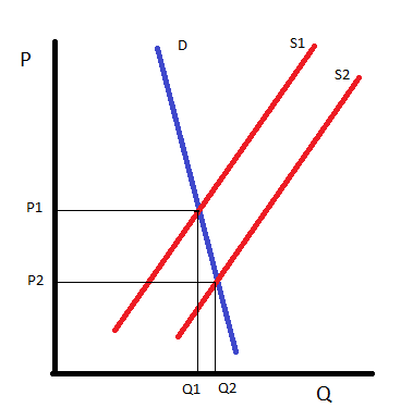
Price elasticity of demand for farm products is very low, 0.40 to 0.20
.
Short-run effects:
- Effect of a bumper crop: Because of price inelasticity of demand, when a farmer produces a bumper crop (moving from S1 to S2), the extra quantity produced is sold for a drastically reduced price, with the irony that the revenues drop drastically.
- Poor crop: Moving from S2 to S1, the price drastically increases, bringing in a much better revenue. So a farmer may be better off financially with a poor crop than a bumper crop.
Long term effects:
- Farming is a declining industry: Demand is not keeping up with supply. The technological advances being made in agriculture (DNA work, new varieties, new farm management theories etc) are producing relatively large increases in supply, but the demand for agricultural products isn't changing much, being mainly fuelled by population increase. And with the well fed, well educated population, increase isn't really happening much.
- The case for and against minimum wage
-

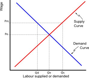
One of the consequences of minimum wage legislation is that it produces a situation the same as a price floor. Assuming cet. par., a price minimum (Pm) which is above the equilibrium price (Pe) will produce an over-supply (Qd to Qs) of labour (unemployment) as more workers are attracted to the higher wages (Qe to Qs) and businesses are motivated to cut staff (Qe to Qd) to maintain profits.
Definitions of business units
Definition, pros and cons of different business units
| Business type | Money Capital | Set up | Business risk | Liability | Management | Other Pros | Other cons |
|---|
| Sole proprietor | Limited to what the sole proprietor actually owns, so expansion is difficult | Easy to set up | High, banks reluctant to lend | Unlimited: risking personal assets as well as business | Owner has to do everything | - Owner very connected to business
- Great motivation to manage successfully
| - Owner does everything, no specialisation
|
| Partnership | Limited to what the partners own. Expansion difficult, but not as difficult as above | Easy to set up | Banks more comfortable to lend money, but still not entirely comfortable | Unlimited: partners risk personal assets as well as business | Some form of management specialisation | - More finance available due to the partnership
- More able to expand the business due to involvement of more partners (investment & labour)
| - Possibility of management conflict - who is responsible for what
- Possibility of conflicting management directions
- Sudden removal of a partner may be detrimental to the business (eg: death, disability, divorce etc)
|
| Proprietary Limited Company | Easily raised through selling shares and bonds | Some legal red tape and costs to set up | Low: banks willing to lend | Limited: owners' assets are shielded, the liability is limited to the amount of their shares and bonds | Management can specialise | - Company is a legal entity, therefore not affected by changes in ownership, is in theory immortal
- Company can easily expand due to ease of finance
| - Disconnect between ownership and control (owners and company officials may be motivated in opposite directions)
- Dodgy company officers able to protect their assets from suing
- More legal requirements to run, more red tape
|
Firm
A business or organisation that operates plant.
Industry
A group of firms that produce the same or similar products.
Plant
The physical establishment used to conduct business. Examples: a shop, cafe, mine, farm etc.
Short-run Production


Short term: period of time where at least one factor (usually plant) is fixed.
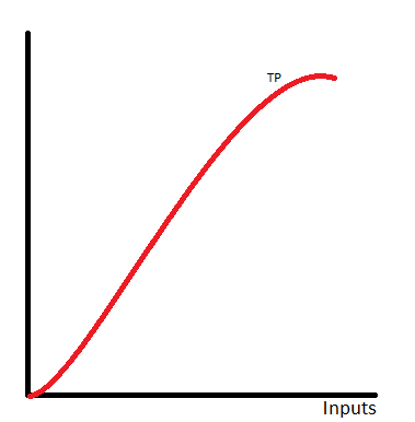
- Total product
The total number of widgets a producer makes (Q).
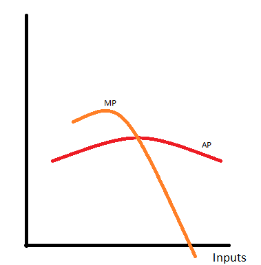
- Marginal product
The change in the number of widgets (ΔQ) for one extra unit of input, ie: MP = ΔQ / ΔInputs
- Average product
The total number of widgets produced divided by the total number of units of input, ie: AP = Q / Inputs
- Fixed costs
(FC or TFC) Those costs, that for a certain defined time period don't vary with output. Usually plant related. Usually stuff like: insurance, rent of premises, wages of key personnel, the normal profit of the entrepreneur etc.
- Average fixed costs
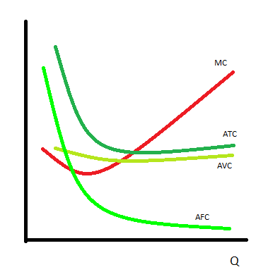
Fixed costs averaged out over the total production, ie: AFC = TFC / Q
Note that AFC approaches zero as the number of widgets produced increases.
- Variable costs
(VC or TVC) Costs that vary with output.
- Average variable costs
Variable costs averaged out over the total production, ie: AVC = TVC / Q. Curve is a typical bowl shape. Minimum is cut by the marginal cost curve.
- Total costs
(TC) The sum of the fixed and variable costs, ie: TC = TFC + TVC
- Average total costs
(ATC) the total cost per unit of production, ie: ATC = TC / Q or ATC = AFC + AVC
Note that TC approaches AVC as production increases. This is because AFC approaches zero as production increases. The marginal cost curve cuts the minimum.
- Marginal cost
The change in total costs per change in total production, ie: MC = ΔTC / ΔQ. Note: the MC curve cuts both the AVC and ATC curves at their minimum.
- Marginal Revenue
The extra revenue generated by the production of one more unit of production, ie: MR = ΔTR / ΔQ
Marginal revenue is zero at the point of unit elastcity, ie: if PED = 0, MR = 0
- Average revenue
The average revenue is AR = TR / Q, which may or may not equal price.
Average revenue curve is usually the demand curve.
- Diminishing marginal returns
-
Also known as diminishing marginal product, or law of diminishing returns or law of diminishing marginal productivity.
As successive units of a variable resource are added to a fixed resource, beyond some point the resulting marginal product associated with each additional unit of input of the variable will decline
. That is, at some level of production, if you add another unit of a resource, then the change in the amount produced will be less than the unit added before it.
DMR is a short-run concept.
Uses the assumption that all units of the input looked at are of the same quality.
DMR kicks in at some point because of the short-run restrictions due to fixed plant.
Example: Farmer using fertilizer. First bag produces some increase, next bag a bigger increase, the third bag is the amount that is optimal and produces the biggest increase. From this point on DMR sets in. Each extra bag of fertilizer will increase the crop a little less than the third bag did, getting to the point that an extra bag of fertilezer will actually produce a slight drop in the crop. In this case, the fixed plant restriction is the acreage of the crop.
DMR cuts in from where the slope of the MC/MP curves are zero.
Shifts in the cost curve:
- Improving technology will shift cost curves down, and product curves up, and change the production quantity at which the AVC and ATC hit their minimum.
Justification for the shape of the TVC (and TC) curve: diminishing marginal returns. In the first part of the graph, MP is increasing (MC decreasing), so the rate of change of Q is increasing. Adding an extra unit of input increases the quantity of widgets produced by a greater and greater amount. When the slopes of the MC and MP curves are equal, that's when the change in the amount of widgets is greatest, and close to this point, each unit of input produces around about the same increase in production of widgits. After this point, DMR kicks in. An extra unit of input will not increase the amount of widgets produced as much as the previous one did. As this continues, it gets to the point where MP = 0, that is: an extra unit of input does not change the number of widgets produced at all. Beyond this point, MP is less than zero, which means that adding an extra unit of input will decrease the amount of widgets produced. In fact, each unit of input added from this point on will have an increasing negative effect on the quantity of widgets produced.
Example of above: Consider a plant that produces widgets with a number of different machines at each step. Going from zero to one worker, production would start, a certain number of widgets would be produced. However, to make them, your one worker will have to switch from machine to machine to machine. Adding a second worker would more than double the number of widgets produced, because as well as being now able to run two machines at once, there will be the beginnings of specialisation of labour. One worker could specialise in one set of machines, while the other specialises in the rest of them. Adding more workers increases the efficiency of the use of the plant, narrowing the specialisation of each worker. At some point, DMR sets in. Putting on extra workers still increases production, but not as much. For example, you may be at the point where workers are waiting for someone else to finish on a machine before they can start their work. Adding workers beyond the point where they have a positive effect on production volumes may start to introduce stuff like overcrowding, people getting in the way of production, slowdowns due to the extra management effort to manage a larger workforce.
The MC curve cuts the TVC (and hence the TC) curves at their minimum.
The AP curve is the horizontal mirror image of the AC curve, and the MP curve is the horizontal mirror image of the MC curve.
Where the MP curve crosses the x-axis, that is where the TP curve is zero. That is, any additional units of input at this point does not make any difference to the quantity of widgets produced. Where the MP curve is below zero, that is where the TP curve has a negative slope, that is, additional inputs at this point have a detrimental affect on the number of widgets produced, ie: the number of widgets produced is less.
Think of the MP curve as the slope of the TP curve, and the MC curve as the slope of the TC curve.
Costs are plotted against production volumes (Q), whereas TP and MP are plotted against inputs.
Long-run production


Plant size is now a variable.
The long-run average cost curve is also known as a company's planning curve.
Economies of scale: The forces that reduce the average cost of producing a product as the firm expands the size of its output in the long run
.
- Labour specialisation: Jobs can be subdivided, allowing workers to become specialists in some aspect of the job. Specialisation means that they get better at what they do, more time-efficient. They don't waste time switching from job to job. Those with specialist skills (say fitters and turners) can concentrate on what they do best.
- Managerial specialisation: A administrator at a small plant may be underutilized if he is managing half a dozen people when he is able to manage say 25. Production staff in this case can be increased without spending more on administration costs. Similarly with labour specialisation, the management tasks can be split up for specialists.
- Efficient capital: Larger firms are able to use more expensive, more efficient capital. For example, CUB may be able to afford and run a 1000 bottle a minute filler, running it most of the time, but a micro-brewer won't have the capacity to efficiently use the filler.
- By-products: Larger firms are able to either install capital that will process by-products to manufacture other products or have the volumes of the by-product such that they can sell it to other firms who may use it as viable inputs for their production. Smaller firms may have to dispose of this by-product.
Diseconomies of scale: As plants become even larger, the long-run average cost curve (long-run ATC) may show an increasing average cost per product. This is mainly due to management problems. As the scale of the operation increases, managers become increasingly out of touch with the production, and the increased complexity may lead to a manager not having enough understanding of the process to make an informed decision. Authority must be delegated. There are problems of coordination and bureaucratic red tape. Increasing the plant size becomes very expensive as they grow massive, for example, a larger plant will need a larger block of land, which may be more difficult to buy, hence more expensive.
In the first graph, the average cost curves for 4 different plant sizes are shown. In this case, the long-term average cost curve would be the combination of ATC-1 from 0 to Q1, ATC-2 from Q1 to Q2, ATC-3 from Q2 to Q3 and ATC-4 from Q3, resulting in a "lumpy" long-term ATC curve. The indicated quantities (Q1, Q2 and Q3) are the production levels where the firm should be considering expanding their plant to the next level.
The second graph shows the long-term average cost curve (in red) for many plants. As the number of possible plants increase, the long-term ATC curve becomes smoother.
The minimum efficient scale (MES) is the smallest level of output that achieves the minimum long-term average costs. It is the quantity Qmes in both graphs.
The shape of the long-term ATC determines the structure and competitiveness (ie: if there are a lot of companies in the industry, then it is competitive) of an industry. For example, if the MES occurs at relatively low production volumes, then an industry will be made up of many small firms. If the MES is at high volumes, then the industry will have a few large firms. If the long-term ATC curve is fairly flat at the minimum cost (like a flat-bottomed dish or plate, rather than being U-shaped), then the size of the firms in the industry will be reasonably diverse (Note: plants in the flat bottom part of the curve are experiencing constant economies of scale, where expanding the plant size will give the same minimum ATC). In the case of a natural monopoly, the MES quantity is larger than the market for the product, with the most efficient system being a single firm producing the product at some point to the left of the MES, with volumes matching the market demand. Real-life examples of a natural monopoly: railway lines, gas pipelines.
Market Failure
Governments provide stuff that the free market won't (public goods), eg: Police force, fire-fighting, ambulance etc
Government provides legislation to control externalities, eg: pollution
Asymmetric information: Seller knows far more than the consumer about his product and alternatives, and uses that to charge a higher price than what it's worth.
ACCC (Australian Competition and Consumer Commission) is the government regulator when it comes to knocking anticompetitive behaviour on the head. Consumer protection policy.
Not all bad behaviour can be efficiently knocked on the head (similar to police can't nab all speeders). Arguement similar to the marginal benefit / marginal cost trade-off.
Trade Practises Act


 Market period or Immediate period: This is the period immediately after a price change (P to P'). The producers have no chance to make any changes to adjust the quantity supplied to the new price, so it stays at Q. An example: a producer brings a truck-load of tomatoes to the farmers' market. Because demand is high, he sells the lot, however he can't produce more there and then to satisfy demand. The truck-load is all he's got for now. Price elasticity of supply is almost perfectly inelastic.
 Short run: In the short-run, the producers are starting to change their production to suit the new demand. At least one, but not all of their inputs have changed to meet the increased demand.
  Long run: Suppliers have had all the time they need to adjust to the new level of demand. Producers have done what they can to meet the new demand.


 Constant cost: As above. Entry/exit of firms does not affect resource prices. The long-term industry supply curve is horizontal to the Q axis. That is, supply is perfectly elastic.
 Increasing cost: Entry into the market causes the resource costs to increase, as firms bid-up the price. The long -term industry supply curve has a positive slope.
 Decreasing cost: Apparently this does happen. One example: mines open up in an area. The first mine to open up has to use relatively more expensive transport to get their ore to market. As more mines open up in the area, it may become convenient to put in a rail line, decreasing transport costs. In this case, the long-term industry supply curve has a negative slope.